Lifting Analysis of Transformer Tank Using Remote Points in ANSYS
Introduction
Transformer tanks are critical components in electrical power systems, and their structural integrity during lifting operations is paramount for safety and reliability. During manufacturing, transportation, and installation, transformers must be lifted using designated lifting lugs or bollards. A proper lifting analysis ensures that these lifting points can safely support the transformer’s weight without excessive deformation or failure.
In this blog post, we’ll explore how to perform a suspended condition lifting analysis of a transformer tank using ANSYS Mechanical, with a specific focus on the application of Remote Points—a powerful feature that simplifies constraint definition and accurately represents lifting cable connections.
What is Lifting Analysis?
Lifting analysis is a structural finite element analysis (FEA) performed to evaluate the stresses, strains, and deformations in a structure when it is suspended by lifting points. For transformer tanks, this analysis helps engineers:
- Verify that lifting lugs can safely support the total weight.
- Identify stress concentrations and potential failure points.
- Ensure compliance with design codes and safety standards.
- Optimize lifting lug design and placement.
- Validate that deformations remain within acceptable limits.
Understanding Suspended Condition Analysis
The analysis methodology presented here simulates the transformer tank in a suspended equilibrium condition—that is, when the tank is already lifted and hanging stationary from the lifting cables.
This represents the state where:
- The tank is fully supported by lifting cables at designated lifting points.
- All forces are in equilibrium (no acceleration).
- The structure experiences maximum sustained loading.
- Cable tensions equal the distributed weight of the transformer.
This approach is widely used in industry as it provides a clear, direct assessment of structural stresses while the transformer hangs suspended during transportation or installation.
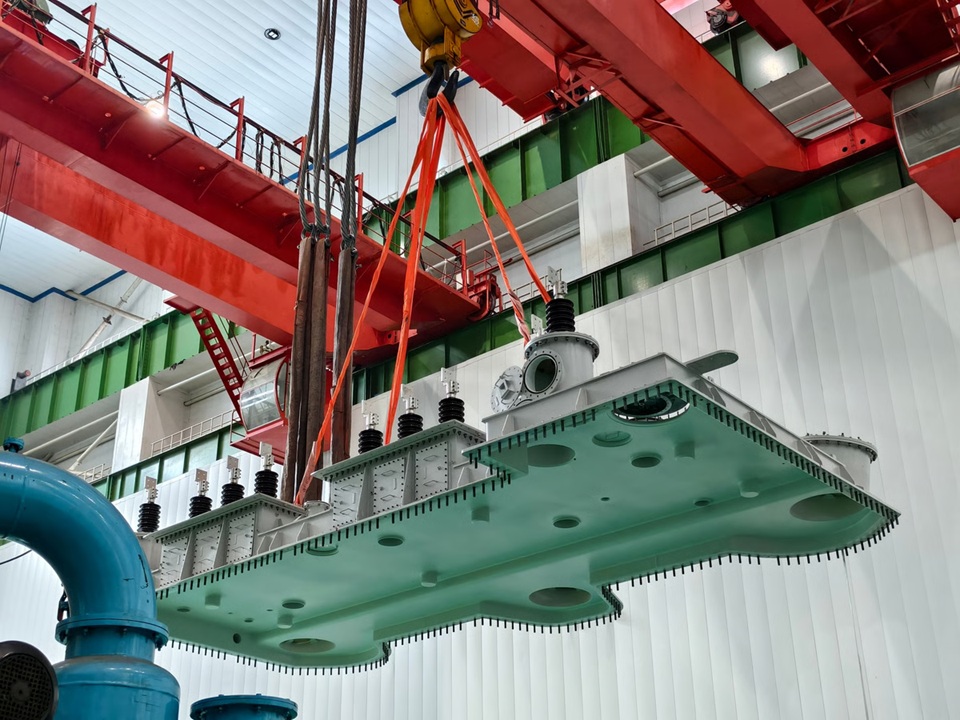 Figure 1: Suspended equilibrium condition diagram.
Why Use Remote Points?
Remote points in ANSYS are powerful tools that allow you to apply constraints at a reference location that is connected to a set of nodes or surfaces through kinematic coupling equations. They are special nodes in the model that represent a collection of points or a portion of the structure, helping to simplify complex behaviors by reducing multiple degrees of freedom to fewer, manageable ones.
How Remote Points Work
Remote points function through Multi-Point Constraint (MPC) equations that manage the relationship between independent and dependent degrees of freedom:
- The remote point acts as an independent node in space coordinates.
- The scoped geometry (lifting hole surface) contains dependent nodes.
- MPC equations link these together, transferring constraints from the remote point to the geometry.
- Dependent degrees of freedom are eliminated from the system, simplifying the solution process.
This mechanism ensures that constraints applied remotely are correctly transferred to the actual model geometry while maintaining physical accuracy.
Methodology
1. Geometry Preparation
Start with a 3D CAD model of your transformer tank. The model used in this analysis was created in Creo and imported into ANSYS.
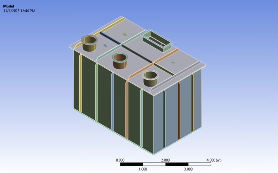 Figure 2: Cleaned CAD geometry ready for analysis.
Essential components to include:
- Main tank body (shell)
- Lifting lugs with mounting pads
- Major structural reinforcements
- Base plate or support structure
Note: Remove small features like bolt holes if they’re far from critical regions. Keep the lifting lug geometry detailed as it’s the region of interest.
2. Material Definition
Define material properties in ANSYS Engineering Data.
- Material: Structural Steel (typical for transformer tanks)
- Young’s Modulus: 200 GPa
- Poisson’s Ratio: 0.3
- Density: 7850 kg/m³
- Yield Strength: 250 MPa
3. Contact Definitions
For multi-body assemblies, create appropriate contacts between components.
- Contact Type: Bonded (This simulates a welded connection).
4. Meshing Strategy
A proper mesh is crucial for accurate results at the lifting points.
- Lifting lug region: Element size: 2-5 mm (fine mesh). Use the “Sphere of influence” method around lifting holes.
- Tank body: Element size: 20 mm.
5. Creating Coordinate Systems
Create coordinate systems at the lifting hook position. This is the point where the lifting cables (slings) converge and connect to the crane hook.
Understanding Sling Geometry: In practical lifting operations, multiple slings connect the lifting lugs to a common lifting hook above. The geometry involves:
- Slinging angle: The angle between the sling and the vertical axis (typically 60° as per standard practice).
- Lifting angle: The angle at the hook where slings converge.
- Hook height: Vertical distance from lifting lug to the hook convergence point.
 Figure 3: Sling geometry reference (CBIP Manual: Section CC).
Steps to create Coordinate System:
- Select the internal surface of the lifting lug/eye or surface of the lifting bollard.
- Insert → Coordinate System.
- This will create a Coordinate System at the centroid of the lifting lugs (x,z).
- Add a vertical offset for the location of the Lifting hook (y). (If hook height is unknown: Calculate it from sling length and angle).
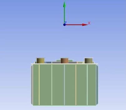 Figure 4: Coordinate System created at the theoretical hook convergence point.
6. Creating Remote Points - The Key Step
Step 1: Insert Remote Point Right-click on Model → Insert → Remote Point.
Step 2: Define Scoping Configure the remote point settings as follows:
- Scoping Method: Geometry Selection.
- Geometry: Select the inner cylindrical surface of all lifting holes (can select multiple faces for all lugs).
- Coordinate System: Select the coordinate system created in Step 5 (at hook position). (Coordinates will automatically populate X, Y, Z = 0 mm relative to selected coordinate system).
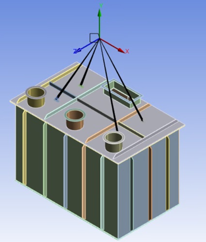 Figure 5: Defining the Remote Point in ANSYS.
7. Applying Loads
The suspended condition analysis requires applying all downward forces that the lifting system must support.
- Load: Standard Earth Gravity
- Application: Insert → Standard Earth Gravity
- Direction: Negative Y-axis (or Z-axis, depending on your coordinate system)
- Magnitude: 9.81 m/s² (automatically applied)
What this does: It applies gravitational acceleration to all bodies. The weight is calculated automatically (Force = Mass × 9.81), where Mass comes from Volume × Density.
Note: This blog focuses on empty tank lifting, so we only use Standard Earth Gravity. Additional loads of Oil and Active Part can be applied on the base plate if required.
8. Applying Boundary Conditions
At the remote point, we need to simulate the hook holding the system stationary.
- Insert → Remote Displacement
- Set ALL degrees of freedom to ZERO:
- X Displacement: 0
- Y Displacement: 0
- Z Displacement: 0
- X Rotation: 0
- Y Rotation: 0
- Z Rotation: 0
The remote points represent lifting cable attachment points. Setting DOF = 0 means these points are held stationary in space, supporting the tank.
Solution and Results
Insert the following result items to evaluate the analysis:
Stress Results
Equivalent (von Mises) Stress: This is the most commonly used failure criterion for ductile materials.
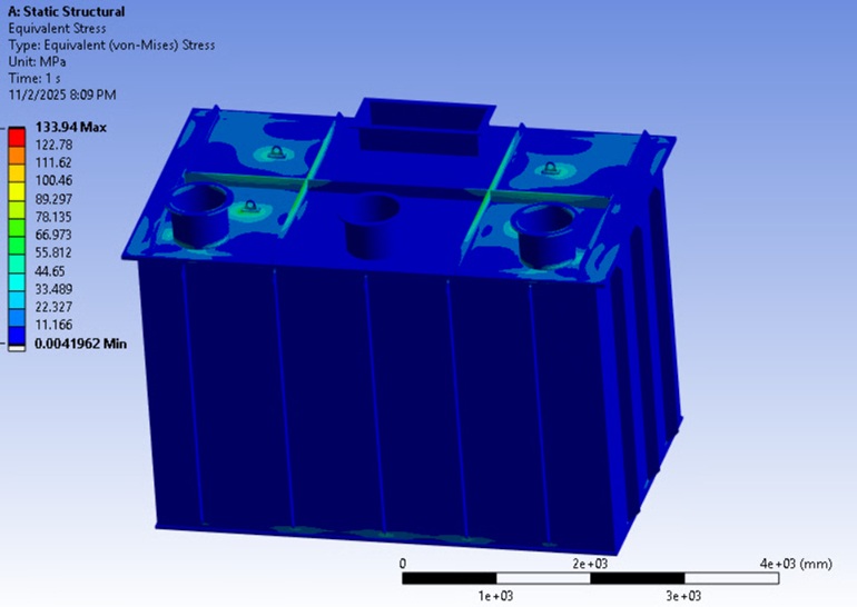 Figure 6: Equivalent (von Mises) Stress distribution.
Deformation Results
Total Deformation: Check the overall displacement of the structure.
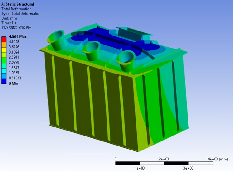 Figure 7: Total Deformation (200% scaled visualization).
Reaction Forces (Validation)
This is a critical step to validate your setup. Insert a Force Reaction probe at each remote point.
- This displays reaction forces in X, Y, and Z directions.
- The Y component (vertical) represents the cable tension.
- The sum of all vertical reactions should equal the total weight of the model.
Validation Check:
First, verify the total mass of your geometry from the properties menu: 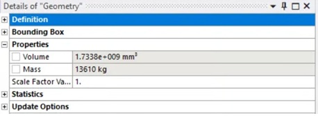 Figure 8: Checking total mass in geometry properties.
Next, check the resultant force from the reaction probes: 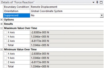 Figure 9: Reaction forces at the lifting points.
Calculation:
- Total weight = $13610 \text{ kg} \times 9.81 \text{ m/s}^2 = 133,514 \text{ N}$
- Reactions in Y (from ANSYS) = 133,460 N
Since $133,514 \text{ N} \approx 133,460 \text{ N}$, the force balance confirms that the model is in equilibrium, the setup is correct, and the results are valid.
What Do the Standards Say?
Ensure your design complies with relevant local and international standards.
CBIP (Central Board of Irrigation and Power) 
CEA (Central Electricity Authority)